



Every peak shaving system has a moment of truth. The building load surges, the meter is climbing toward the monthly maximum, and somewhere in the controller a decision is made - in milliseconds or in the previous midnight's planning run - about whether and how fast the battery should discharge.
Most owners never see that decision. They see the outcome in the demand charge line, and when the outcome is good they credit the battery, and when it is bad they blame the battery. In reality, the battery is the last link in a chain that starts with a measurement and passes through a peak shaving algorithm whose design determines most of the savings.
This article opens that black box: what the control loop actually measures, how the three generations of dispatch logic work, where each one fails, and how to tell whether your system's algorithm is earning its keep. It is the mechanics companion to our articles on peak shaving savings and industrial peak shaving strategies, which cover the value case and the site-side tactics. Here we stay inside the controller.

The Anatomy of the Control Loop
Strip away the branding and every peak shaving controller is the same four-part structure:
A measurement - the site load, read from a meter or current transformers at a defined point. A setpoint - the target demand the algorithm tries not to exceed. An error - the gap between measured load and setpoint, which is the signal the battery must cover. A control action - the discharge (or charge) command issued to the inverter, rate-limited by the PCS rating and the available state of charge.
Four design choices inside that structure separate competent systems from disappointing ones: where the measurement is taken, how the setpoint is chosen, whether the algorithm looks forward in time, and how the state of charge is budgeted. Each is worth understanding, because each is a place where savings quietly leak.
The measurement point matters more than anything else in the specification. The battery can only shave what the meter sees. If the CTs are placed on a feeder upstream of the battery's own charging load, the system will charge during the day and push the measured load above the setpoint with its own consumption - the classic self-defeating installation. If the billing meter and the control meter are different devices with different accuracies, a 1 to 2 percent discrepancy at a 500 kW peak is 5 to 10 kW of unbudgeted error. The control measurement should be at the point of interconnection, same side, same accuracy class as billing, and the algorithm must net out its own charge load.
Generation One: Reactive Threshold Control
The simplest algorithm - and still the most common in entry-level products - is pure reaction. Measure the load. If it exceeds the setpoint, discharge at the excess. If it falls below, stop, and later, charge.
It works, and for well-behaved loads with slow peaks it works well. An office building whose demand ramps over forty minutes gives a reactive controller plenty of warning implicit in the ramp itself.
Its failure modes are structural, not tunable. A step load - a chiller bank starting, a crane regenerating, a welder firing - crosses the setpoint faster than the control loop reacts, and the peak books itself in the one or two intervals before the battery catches up. Worse, the reactive controller has no forward view of energy: it discharges freely at every excursion and can arrive at the real afternoon peak with a depleted battery. Reactive control handles the peaks it expects by accident and misses the ones that matter.
The refinements that make generation one usable are hysteresis and deadband - discharging only above setpoint plus a small margin, releasing below setpoint minus another margin, so the system does not chatter around the target and burn cycles on noise. Add a ramp on the exit - discharging down over a minute rather than stopping instantly - and the control chattering that plagues cheap installs mostly disappears.

Generation Two: Budgeted Reactive Control
The intermediate generation adds the missing resource view: the algorithm tracks available energy and spends it deliberately.
The state of charge is budgeted across the day. A morning reserve is held regardless of early excursions. Discharge authority above the setpoint scales with remaining budget - full power while the budget is deep, tapering as it thins. And charging is scheduled into known-cheap, known-quiet hours rather than opportunistically whenever the load dips.
This single change fixes the exhaustion failure: the battery no longer spends its energy on the third-largest spike of the morning and arrives empty at the largest peak of the afternoon. The budget is crude - usually a linear allocation across the operating window - but it converts the battery from a reflex into a resource manager.
Generation Three: Forecast-Assisted Dispatch
The third generation adds a forward view: a predicted load curve, typically built day-ahead and updated intraday, from which the algorithm plans the full state-of-charge trajectory in advance.
With a forecast, the dispatch decisions change character. Pre-discharge becomes possible - deliberately running the site load down before the predicted peak so the battery is not caught mid-charge when it arrives. Charging windows are chosen against both the forecast valley and the tariff, not just one. And the look-ahead window answers the question reactive control cannot: not just "is the load high now" but "is this excursion worth spending the reserve on, or is a bigger one three hours away."
The forecast does not need to be sophisticated to help. A persistence model - today looks like the comparable day last week, adjusted for weather - captures most of the value in buildings with routine-shaped loads. The marginal gain from machine-learning forecasts is real but concentrated in sites with volatile, weather-driven or schedule-irregular loads. Our AI dispatch article covers that upper tier, including how degradation cost enters the optimisation; this article's point is simpler - even a modest forecast changes the shape of the SOC trajectory for the better, because planning beats reaction at equal information quality.
Choosing the Setpoint
The setpoint is where the money is, and there are three schools.
A static setpoint - fixed at, say, 90 percent of the historic maximum - is simple and transparent, and wrong the month the load grows. Rolling-maximum adaptation - tracking the recent maximum and backing off a margin - self-adjusts but ratchets upward after anomalies, locking in a high target. Percentile-based selection - targeting a demand level that the battery can defend on, say, 95 percent of days - is the most honest formulation, because it makes the trade explicit: on the worst 5 percent of days, the peak will exceed the setpoint, and the model should say so.
That last honesty matters for the demand charge itself. In markets where the billed demand is the single highest interval of the month, one miss resets the whole month; the algorithm's real objective is not average performance but zero misses, which pushes toward conservative setpoints and deep reserves. Where the billing averages the top intervals, or uses ratchets, the optimum shifts. The tariff mechanics - not the algorithm marketing - should set the aggressiveness.
Guardrails: The Layer Above the Objective
Production systems sit a guardrail layer above the optimisation, and its rules are non-negotiable in the correct design:
Minimum state of charge that arbitrage and shaving cannot breach, reserved for outage cover or contractual obligations. A reserve release order - when the battery is nearly empty and the load still exceeds the target, discharge down to the floor rather than hoarding a reserve that will not be needed. Exit ramps that bring discharge to zero smoothly, so the site load never sees a step. And a hard ceiling on daily cycle count or throughput, because an algorithm optimising today's demand charge without a degradation term will happily cycle the battery into early replacement - the warranty knows the duty cycle even if the algorithm does not.
Five Ways Tuned Systems Fail in the Field
The patterns repeat across sites, and each is a checklist item.
The setpoint is set below what the battery can defend, so the system exhausts early and misses anyway - a target between the battery's capability and the load's behaviour was never achievable, and the fix is a sizing conversation, not a tuning one. The SOC is spent before the peak - usually a missing budget layer or a charging window that overlaps the morning ramp. Holidays and shutdown weeks - the algorithm holds a full reserve for a peak that will not come, and the arbitrage layer sits idle; calendar awareness is cheap and often missing. The tariff clock is wrong - the system shifts load against a schedule that no longer matches the utility's seasonal rates, a five-minute fix discovered only in the bill. The measurement is single-point - one CT, one meter, no cross-check - so a CT failure or drift silently disables the control loop while the system reports healthy.
How to Audit Your Algorithm
Three questions, answerable from data you already own.
What is the peak hit rate - the share of billing-relevant days on which the monthly maximum stayed at or below the target? Below the mid-nineties in percent terms means the setpoint or the budget is wrong. What is the SOC utilisation - how much of the purchased energy actually gets cycled on a typical day? A system deeply discharged twice a month is sized wrong or budgeted too conservatively. And what happened on the worst day of each month - the one interval that set the bill? Trace those days: nearly every one traces to one of the five failure modes above, and the trace is the tuning roadmap.
The uncomfortable summary is that the algorithm rarely fails mysteriously. It fails at the measurement point, at the setpoint, or at the SOC budget - three places that are all visible in data the system already records. Owners who look at those three regularly keep their peak shaving algorithm honest; owners who look only at the demand charge discover the drift a year late, in the bill.

MECC 50KW 108KWH BESS Battery Energy Storage System
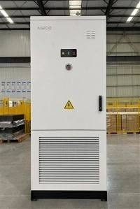
The MECC 50kw 108kWh Battery Energy Storage Cabinet is a high-capacity energy storage solution designed for industrial and commercial applications. Featuring 345.6V, 314Ah lithium iron phosphate (LiFePO4) battery, it ensures long-lasting, safe, and efficient energy storage.
High-efficiency 50kW/108kWh Industrial and Commercial Energy Storage System (C&I ESS). Features LiFePO4 battery, peak shaving, and smart EMS. Reduce operational costs and ensure power backup. Inquire for custom BESS solutions.
Designed with a compact footprint of less than 1.2 square meters, this 108kWh cabinet features a pre-integrated all-in-one design, reducing on-site installation time by 40% compared to modular rack systems.