





Two systems with identical batteries, identical PCS and identical tariffs can produce savings that differ by 30%. The variable is not hardware. It is the peak shaving algorithm deciding, second by second, when to discharge and how much.
Vendors describe this layer in marketing language - "AI-powered," "self-learning," "predictive." What matters is more concrete: what the controller measures, what it forecasts, what it optimises, and what it does when the forecast is wrong.
This is a tour of the decision chain inside a commercial storage controller, and of the design choices that separate a system that delivers its modelled savings from one that quietly underperforms.
The problem the algorithm is solving
Stated formally, the controller minimises billed demand over a billing period, subject to constraints:
Power cannot exceed the PCS rating, and ramp rates are finite.
Energy cannot exceed what is stored, and state of charge must stay within limits.
Round-trip efficiency losses mean discharging 100 kWh returns roughly 85–90 kWh to the site.
Cycling has a cost - degradation - so not every avoided kilowatt is worth avoiding.
The future load is unknown, so every decision is made under uncertainty.
That last constraint is what makes the problem interesting. If the load were known in advance, peak shaving would be a straightforward optimisation. Because it is not, the algorithm is fundamentally a forecasting problem wearing a control-theory costume.
The five-stage decision chain
Every commercial controller, however it is marketed, runs the same loop.
1. Measurement. Site meters and CTs sample at one-second to one-minute resolution. The controller computes real power, and often reactive power, at the point of common coupling.
2. Interval projection. This is the step most often underestimated. Utilities bill demand on the average power over a 15-minute (or 30-minute) interval, not the instantaneous value. A controller that reacts to instantaneous power will over-discharge early in the interval and run out of energy before the interval ends.
The correct approach is to track the accumulated energy within the current interval and project the end-of-interval average:
projected average = (energy so far + expected energy for remaining seconds) ÷ interval length
Discharge is triggered when the projected average approaches the target, not when instantaneous power does.
3. Forecast. A short-horizon load forecast - typically 15 to 60 minutes - predicts whether a new peak is likely, and how large. Simple implementations use persistence (assume the last hour repeats). Better ones use day-type profiles plus weather and production schedules. The best blend a physical model with a learned residual.
4. Decision. The optimiser or rule set chooses a discharge setpoint for the next control step, subject to SOC, power and degradation constraints.
5. Verification. The controller logs what it intended, what it commanded and what the meter measured. This record is what makes performance claims auditable - and what exposes algorithms that only work in the demo.
Four algorithm families
Rule-based threshold control. The workhorse. If projected demand exceeds a threshold, discharge the difference; if it falls below threshold minus a deadband, stop. It is transparent, cheap, deterministic and easy to commission.
Its weaknesses are equally clear. It cannot anticipate a peak that has not yet started, so it always responds one interval late. It has no notion of energy budget across the day, so it can exhaust the battery on a morning spike and have nothing left for the afternoon peak that actually sets the ratchet. And without hysteresis it oscillates around the threshold, wasting efficiency.
Forecast-based peak shaving. Adds a load prediction so the controller can pre-discharge before a forecast peak and hold reserve for later. This is where most of the practical improvement lies. A modest forecast with a conservative safety margin outperforms a perfect rule-based controller, because it converts a reactive problem into a scheduling one.
Model predictive control (MPC). At each step, solve an optimisation over a rolling horizon - typically four to twenty-four hours - with forecasts, tariff structure, SOC dynamics and degradation cost in the objective. Execute the first action, then re-solve.
MPC handles multi-objective dispatch naturally: demand charges, TOU arbitrage, solar self-consumption, demand-response obligations and reserve requirements can all sit in one cost function with weights. It also degrades gracefully - when forecasts are poor, the receding horizon corrects.
The cost is computational and engineering effort. MPC needs a credible model of the plant, a reliable forecast, and tuning of the objective weights. A badly tuned MPC can be worse than a well-tuned rule set, particularly if the degradation penalty is set too low and the controller cycles aggressively for marginal savings.
Reinforcement learning. Increasingly offered, rarely necessary. An RL agent can learn a dispatch policy from historical data without an explicit plant model. In practice, most deployed systems use RL as a tuning layer - adjusting thresholds or reserve margins - rather than as the primary controller. The reason is accountability: a deterministic controller can be explained to a utility, an insurer or an asset owner. A learned policy that behaves unexpectedly in an unseen condition is difficult to defend.
For most C&I sites, the pragmatic architecture is forecast-based scheduling plus MPC or advanced rule-based execution, with learning used to tune parameters rather than to make the decisions.
The constraints that shape every decision
State of charge is a budget, not a level. The controller should allocate available energy across the day according to the value of avoiding peaks at different times. A morning peak at $8/kW and an afternoon peak that sets the ratchet are not equal, and the algorithm should know the difference.
Efficiency has a price. Discharging 100 kWh to avoid 80 kWh of demand costs 20 kWh of energy plus cycling wear. If the demand charge is low and the energy price is high, discharging can be net-negative. Good controllers include a marginal cost per discharged kWh.
Degradation is a real cost. Every cycle consumes a fraction of asset life. A degradation penalty of a few cents per kWh is usually enough to stop the controller from chasing trivial peaks without materially reducing savings.
Ramp and response time matter. A 500 kW system that takes 30 seconds to reach full output may still miss a fast load step. The controller must model its own dynamics, not assume instantaneous response.
Reserve must be protected. A minimum SOC reserve - typically 10–20% - should be inviolable except during a grid outage or a contracted demand-response event. Controllers that allow the reserve to be raided for arbitrage will eventually be empty when the peak arrives.
Multi-objective priority: the stack that prevents conflict
A modern C&I controller is usually managing five objectives at once. Without an explicit priority stack, they fight each other.
A workable hierarchy:
Safety and protection - never compromised.
Ratchet or peak prevention - the highest-value, hardest-to-recover objective.
Demand charge target for the current interval.
Contracted demand-response obligations - these carry penalties.
TOU arbitrage.
Solar self-consumption and export limitation.
Resilience reserve.
The order matters. A controller that treats arbitrage and demand reduction as equal-weight objectives will happily discharge at 10 a.m. for a small price spread and then be unable to shave the 4 p.m. peak. Explicit prioritisation prevents that, and makes the behaviour explainable after the fact.
Seven failure modes you will actually see
Chasing the threshold. No deadband, so the system cycles continuously around the target, wasting 5–8% of throughput in efficiency losses.
Interval-boundary blindness. The controller reacts to instantaneous power, discharges heavily in the first five minutes of an interval, then recovers - producing no billed-demand reduction at all.
Forecast latency. The forecast is updated every 15 minutes but the load step happens in 90 seconds. The system responds after the peak has been recorded.
Rebound peaks. The battery discharges, the site load rises immediately afterwards because the discharge masked it, and the next interval peaks higher than the one just shaved.
Pre-peak exhaustion. Energy is spent on morning peaks, leaving nothing for the event that sets the monthly ratchet.
Control fighting with PV. The storage discharges while the inverter is curtailed, or charges from PV while exporting is restricted - both wasting value. Solar and storage must share one control layer, not two.
Lost history at the month boundary. The current-month peak tracker resets, but the ratchet lookback does not. Controllers that only track the current month systematically mis-target.
Tuning parameters that matter more than the algorithm name
Target demand and how it is derived (fixed, rolling, ratchet-aware).
Deadband, typically 3–5% of rated power.
Forecast horizon and the safety margin applied to it.
Minimum SOC reserve and the conditions that may override it.
Maximum discharge ramp and the PCS response model.
Degradation cost per kWh used in the objective.
Interval length and the utility's exact averaging method.
A rule-based controller with well-tuned parameters will beat an untuned MPC on most C&I sites. Ask vendors for these values explicitly, and ask how they were derived.
Measuring whether it worked
Savings claims require a baseline. Use a documentedmethodology - weather-normalised regression on pre-installation interval data, or a control-group comparison across similar sites - rather than a simple year-on-year comparison, which confounds savings with production changes.
Track four KPIs:
Billed demand versus target, by month.
Peak-setting events avoided, and the margin by which they were avoided.
Discharge energy versus throughput limit, to confirm warranty compliance.
Realised savings versus modelled savings, with variance attributed to forecast error, availability and tariff change.
FAQ
What is the simplest peak shaving algorithm that works?
A forecast-based threshold controller with hysteresis, interval-average projection and a protected SOC reserve. It captures most of the available value at a fraction of the engineering cost of MPC.
Is machine learning necessary?
No. Learning improves forecast accuracy and parameter tuning, which helps. But the core decision problem is well served by deterministic optimisation, and deterministic behaviour is easier to warranty and audit.
How accurate does the load forecast need to be?
Better than the safety margin you are willing to carry. A 10% forecast error typically requires a 5–10% capacity margin to avoid misses, which is why forecast quality translates directly into required battery size.
Why does my system discharge but the bill doesn't change?
Usually interval-boundary handling, a ratchet floor making the savings unreachable, or a baseline that was mis-specified. Check the 15-minute interval data against the controller log before assuming the battery is at fault.
Can one controller manage demand charges, TOU and demand response?
Yes, and it should. Separate controllers with separate setpoints will conflict. Insist on a single EMS with an explicit priority stack.
The bottom line
A peak shaving algorithm is a forecasting system wrapped around a constrained optimisation, executed against a billing rule that averages over fifteen minutes. The differences between vendors lie less in the sophistication of the mathematics than in whether they handle interval averaging, SOC budgeting, ratchet history and multi-objective priority correctly.
Ask for those four things. They determine the savings far more than the label on the box.
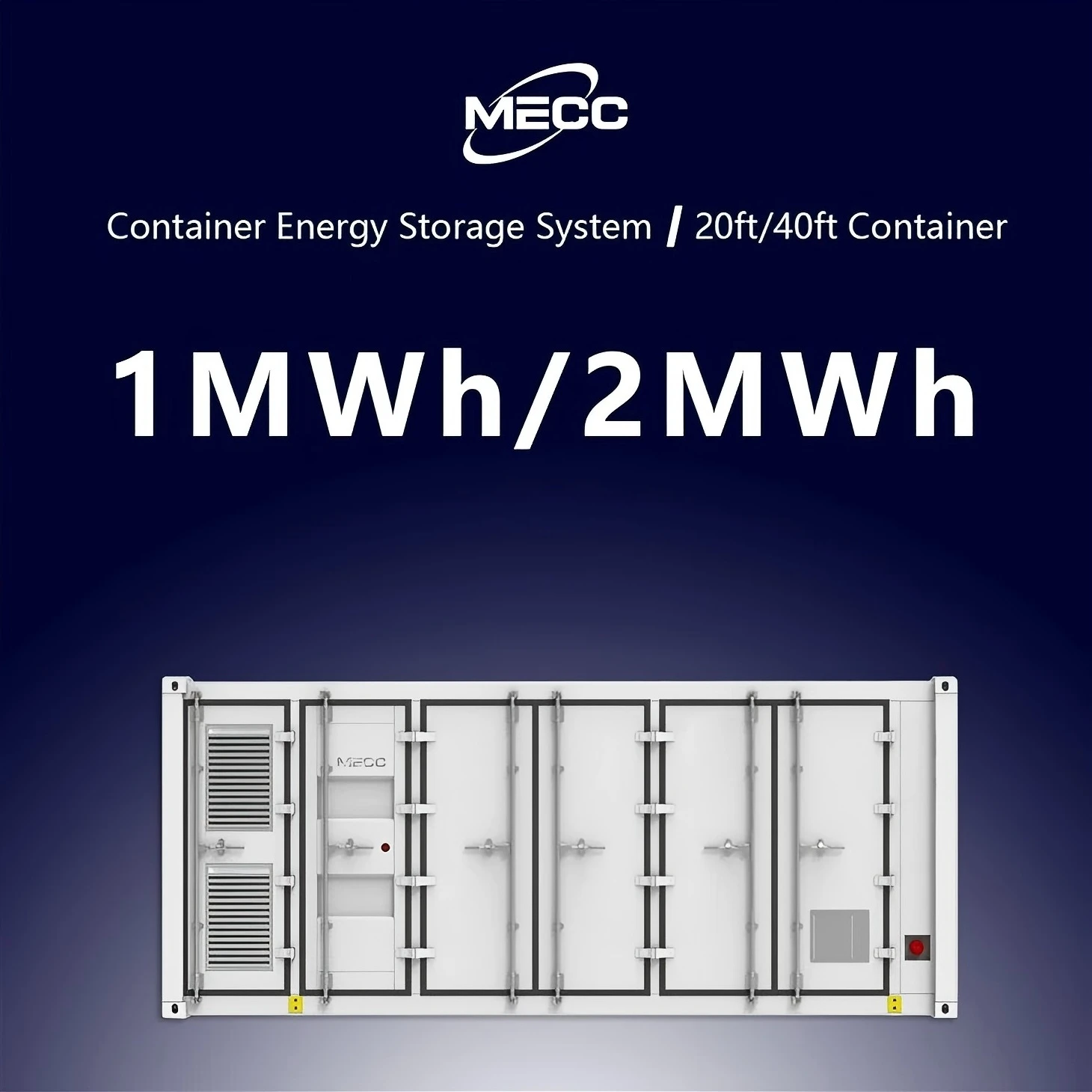
500KW/1MW 1MWh/2MWh Battery Energy Storage System Container
The 500kW/1MW 1MWh/2MWh Battery Energy Storage System Container is a turn‑key utility‑grade energy storage solution housed in standard 20ft or 40ft shipping containers, integrating bidirectional PCS, A‑grade LiFePO4 battery clusters, master BMS, liquid‑cooled thermal management, gas fire suppression, high‑voltage distribution and EMS energy management system with full factory pre‑assembly and pre‑commissioning. Requiring only foundation construction and high‑voltage cable connection for on‑site commissioning, it supports flexible power‑capacity configuration and multi‑container parallel expansion, delivering core capabilities of peak‑shaving and load shifting, renewable energy smoothing, frequency‑voltage grid support, islanded micro‑grid operation and large‑scale emergency backup. Featuring IP54 enclosure protection and comprehensive multi‑layer safety mechanisms, it adapts to diverse harsh outdoor environments, and is widely deployed for ground‑mounted PV power stations, industrial parks, mining operations, island microgrids and grid‑side auxiliary service projects to stabilize grid fluctuations, boost renewable energy utilization and reduce comprehensive energy costs.