





Almost every storage project that underperforms can be traced back to a spreadsheet. Not to the battery, not to the inverter, not to the installer - to a load profile analysis that used monthly bills, averaged away the peak, or sized energy from an annual curve instead of a daily one.
Fifteen-minute interval data is the raw material of a credible design. It is also messier than it looks. This is a practical guide to reading it properly: what to request, how to clean it, which views reveal what, and how to turn the numbers into a power and energy specification.
Get the right file first
Ask the utility or the meter operator for interval data at the native billing interval, in kW or kVA, with a timestamp for every interval, for at least twelve consecutive months. Ideally twenty-four, so you can see a mild year and a severe one.
Confirm these details before analysis:
Interval length. 15 minutes is standard in most markets; some use 30, some 5. Mixing them silently halves or triples your peaks.
Units. kW, kVA or kWh per interval. A column labelled "demand" may be an average power, a maximum, or an energy total.
Meter multiplier. Large services often have CT ratios applied - or not applied. Check the first interval against a known load.
Power factor. If the tariff bills kVA, you need reactive data or at least a power factor assumption. A 0.85 power factor turns a 600 kW load into 706 kVA.
Time zone and daylight saving. Twice a year, an hour is duplicated or skipped. Untreated, this creates a false peak or a gap.
Data flags. Estimated or substituted intervals are usually marked. Filter them; do not let an estimate set your design peak.
Sign convention. Negative values usually mean export. If the site has PV, this matters enormously - the demand charge is based on net import, but the battery may need to absorb surplus.
Clean before you calculate
A short, disciplined cleaning routine prevents most errors:
Rebuild a complete, regular time index at the native interval. Missing rows should be visible, not silently skipped.
Handle DST explicitly - drop or duplicate the repeated hour according to the utility's convention.
Flag and exclude estimated intervals from peak statistics, but keep them for energy totals with a note.
Convert to a consistent unit. Work in kW for power and kWh per interval for energy. For a 15-minute interval, kWh = kW ÷ 4.
Check for negative and zero runs - a stuck meter or a comms outage can produce a flat zero that looks like a very low base load.
Separate sites if sub-metered. Whole-site data includes HVAC, process and EV loads; a submeter tells you which load you can actually shift.
Annotate anomalies. Shutdowns, commissioning periods, COVID-style demand changes, a new production line. A year containing a three-month shutdown will understate the design peak.

Eight views that reveal the design
A single time-series chart tells you almost nothing. These eight views, in this order, tell you most of what you need.
1. The load duration curve. Sort all intervals from highest to lowest and plot against duration. It shows the peak, the base, and how quickly the load falls away. The area under the curve above your target is the annual energy above target - useful context, but not a sizing number, for reasons explained below.
2. The monthly peak map. For each month, plot the day and time of the peak-setting interval. Patterns emerge: summer afternoons, winter mornings, month-end production runs. If peaks cluster in a narrow window, control is easier; if they scatter, the battery needs more reserve.
3. The hour-by-day heat map. 24 columns by 7 rows, coloured by average load. This is the fastest way to see shift patterns, weekend behaviour and lunchtime dips.
4. Weekday versus weekend profiles. Industrial sites often have radically different weekend behaviour. A battery sized on a blended average will be wrong for both.
5. Seasonal profiles. Four representative days, or monthly averages by hour. Cooling and heating loads change the shape, not just the level.
6. The ramp-rate distribution. Compute the interval-to-interval change and plot the histogram. The 95th and 99th percentiles tell you how fast the battery must respond, and whether the PCS ramp rate is adequate.
7. Load factor. Average load divided by peak load. A low load factor - say 0.35 - means a peaky site with good storage economics. A high load factor near 0.8 means a flat site where demand-charge savings will be modest.
8. Overlay with tariff periods and PV. Shade the TOU windows and the solar generation profile on the same chart. This shows whether peaks coincide with expensive periods and whether PV can help shave them.
The five metrics to report
For every site, produce a one-page summary with:
Maximum demand and the date/time it occurred, in kW and kVA.
Base load - the 5th percentile, not the minimum.
Load factor and peak-to-average ratio.
P95 and P99 demand - a more robust design basis than a single maximum, especially if the maximum is an outlier.
Count of intervals within 5% of the maximum - this tells you how "sharp" the peak is. If fifty intervals sit within 5% of the peak, the battery must hold output for a long time; if only two do, it is a spike.
Add the number and duration of excursions above your candidate target. That is the number that sizes the battery.
Sizing energy: use the daily area, not the annual curve
This is the most important technical point in the article.
The annual load duration curve integrates energy above a threshold across the whole year. If you divide that by 365, you get the average daily energy above threshold - which is not what the battery must deliver. The battery must deliver the energy above threshold on the worst day, because that is the day that sets the demand charge or the ratchet.
The correct procedure:
Choose a target demand - the level you want to cap.
For each day, compute the area where load exceeds the target: sum (load − target) × interval duration for all intervals above target.
Rank the days by that area.
Size for a high percentile - the 95th or 99th worst day - not the single worst if it is an outlier, and not the average.
Size power for the maximum gap, not the average gap.
A worked example
Take a site with a 780 kW annual maximum, a 210 kW base load and a load factor of 0.34.
The owner wants to cap demand at 600 kW, so the required power is:
780 − 600 = 180 kW
Now the energy. On the peak day, the load exceeds 600 kW for a total of 2.1 hours across three separate events. The area above the threshold sums to 300 kWh delivered to the site.
Convert that to battery capacity:
Round-trip efficiency 88%: 300 ÷ 0.88 = 341 kWh drawn from the cells.
Usable depth of discharge 90%: 341 ÷ 0.90 = 379 kWh nameplate.
Reserve for forecast error and a second event: add 15% → 436 kWh.
The specification is therefore 180 kW / 435 kWh, roughly a 2.4-hour system at rated power.
Note the gap between the naive answer (300 kWh) and the engineering answer (436 kWh). That 45% difference is where many projects get into trouble - the battery is installed, and on the worst days it runs out before the peak ends.
Also check recovery: after delivering 341 kWh, the battery recharges from the headroom below 600 kW. If the site's load after the event is 400 kW, headroom is 200 kW, and recharging 341 kWh takes 1.7 hours. If events are closer together than that, the reserve must grow.
Nine data traps
Using monthly bills. They hide the interval that set the charge and cannot support any dispatch modelling.
Averaging across a year. It produces a smooth curve that no day resembles.
Sizing on the single maximum. One anomalous interval can add 20% to the specification. Check whether it is repeatable.
Annual duration curve as an energy basis. Overstates or understates depending on the site; always use daily areas.
Ignoring kVA. A 0.85 power factor changes the target by 18%.
Missing DST handling. Creates phantom peaks and phantom gaps.
Export masking. With PV, a negative interval can hide an underlying load that returns when the sun goes down.
Assuming the future looks like the past. Load growth, electrification of heating, and EV charging all change the profile. Ask what is planned.
No sub-metering. Whole-site data cannot tell you whether the peak comes from chillers, process or chargers - and therefore whether it is shiftable.
What to hand to the supplier
A credible tender pack includes: twelve months of 15-minute data in CSV, the tariff sheet, the interval convention, the design target, the calculated power and energy with workings, the top twenty days by area above threshold, and a note on planned load changes.
Suppliers who ask for less than this are guessing. Suppliers who can explain why their sizing differs from yours are worth talking to.
FAQ
How much interval data do I need?
Twelve months minimum, twenty-four preferred. Less than a year will miss seasonal peaks and is not a defensible design basis.
What if the utility only provides 30-minute data?
It is usable for energy and shape, but it understates 15-minute peaks and will understate demand savings. Ask for 15-minute data; if unavailable, apply a conservative margin of 5–10% on power.
Should I use the maximum or the 99th percentile?
Use the maximum for ratchet-exposed sites and the 99th percentile for sites where a rare excursion is tolerable. Report both and state the choice.
Why is the required energy larger than the area above the target?
Because of round-trip efficiency, depth-of-discharge limits and reserve. The area is what the site needs; the nameplate is what you must buy to deliver it.
Can I size from a year of half-hourly kWh readings?
You can estimate, but only if you know the interval convention and have checked the units. In practice, unit confusion is the most common source of a design that is wrong by a factor of four.
The bottom line
Load profile analysis is not a chart-making exercise. It is the process of finding the intervals that set the bill, quantifying the energy above a target on the worst days, and converting that into a nameplate that survives efficiency, depth of discharge and forecast error.
Do it on native interval data, size on daily areas rather than annual curves, and document your workings. The spreadsheet is where the project either works or doesn't.
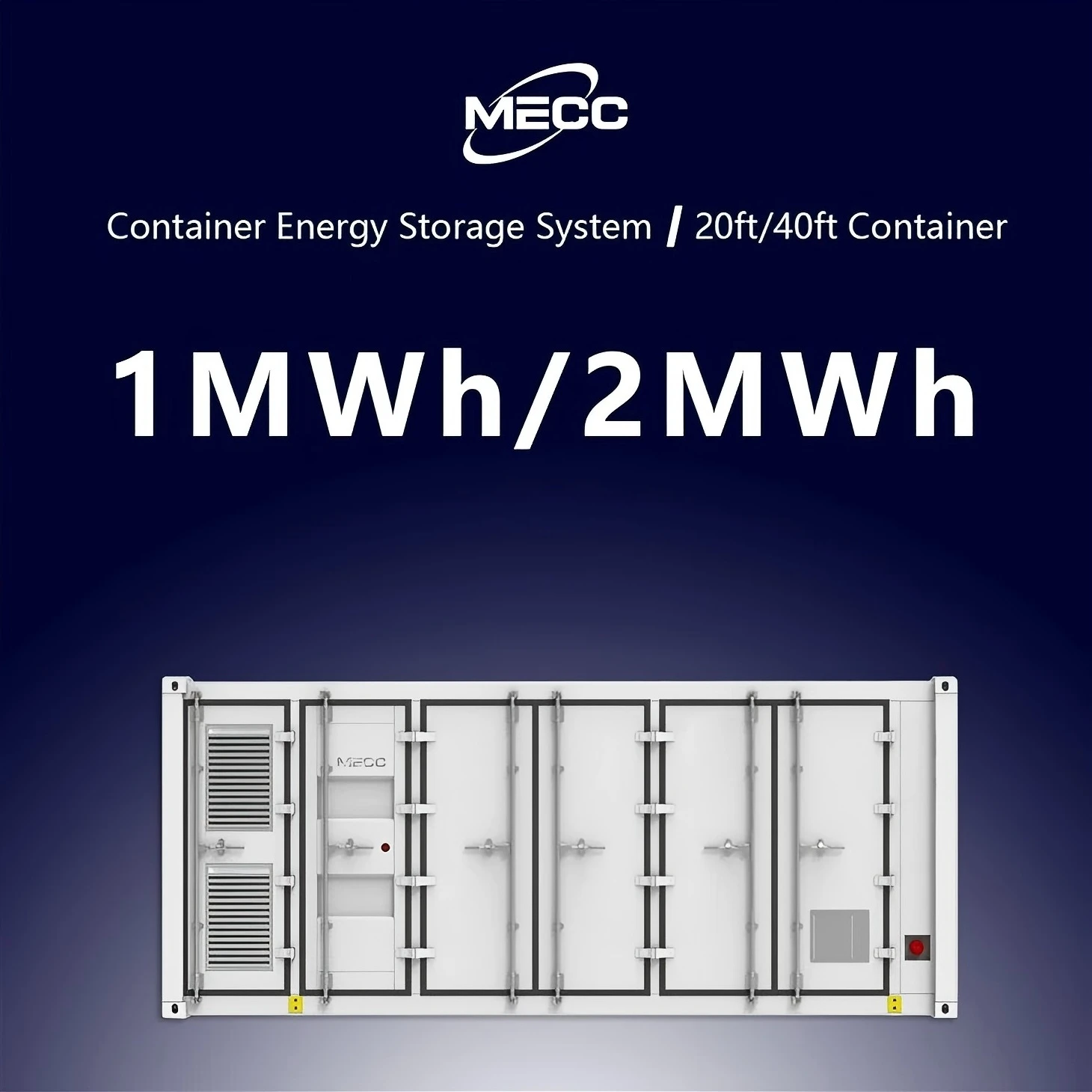
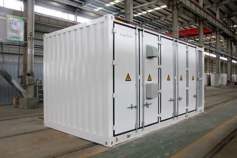
500KW/1MW 1MWh/2MWh Battery Energy Storage System Container
The 500kW/1MW 1MWh/2MWh Battery Energy Storage System Container is a turn‑key utility‑grade energy storage solution housed in standard 20ft or 40ft shipping containers, integrating bidirectional PCS, A‑grade LiFePO4 battery clusters, master BMS, liquid‑cooled thermal management, gas fire suppression, high‑voltage distribution and EMS energy management system with full factory pre‑assembly and pre‑commissioning. Requiring only foundation construction and high‑voltage cable connection for on‑site commissioning, it supports flexible power‑capacity configuration and multi‑container parallel expansion, delivering core capabilities of peak‑shaving and load shifting, renewable energy smoothing, frequency‑voltage grid support, islanded micro‑grid operation and large‑scale emergency backup. Featuring IP54 enclosure protection and comprehensive multi‑layer safety mechanisms, it adapts to diverse harsh outdoor environments, and is widely deployed for ground‑mounted PV power stations, industrial parks, mining operations, island microgrids and grid‑side auxiliary service projects to stabilize grid fluctuations, boost renewable energy utilization and reduce comprehensive energy costs.